If you're using a Linux-based operating system, such as Ubuntu, the Octave PPA is maintained and supported by Octave developers, so you can install the latest stable version of GNU Octave by executing the following lines one by one on the Terminal:
- sudo apt-add-repository ppa:octave/stable
- sudo apt-get update
- sudo apt-get install octave
GNU Octave is a great software for producing high quality plots. In this simple tutorial, we will use Octave, Ipython notebook and Octave kernel for Jupyter to show how this combination of software provides more graphing control and capabilities. The easiest way to install Ipython notebook is by installing Anaconda distribution, which you can do by following instructions here.
We recommend that, you install Octave kernel with pip, just by simply executing the following command in the Terminal:
$pip install octave_kernel
After Installing Ipython notebook and Octave kernel, you can now respectively; use Ipython Notebook, Ipython console and Ipython qtconsole, which you can evoke as follows.
Ipython notebook:
$ipython notebook
After launching Ipython notebook, in its interface, select Octave from the 'New' menu or from the File --> New Notebook.
Ipython console:
$ipython console --kernel octave
Ipython qtconsole:
$ipython qtconsole --kernel octave
Alright, now let's use Ipython notebook to do some graphing.
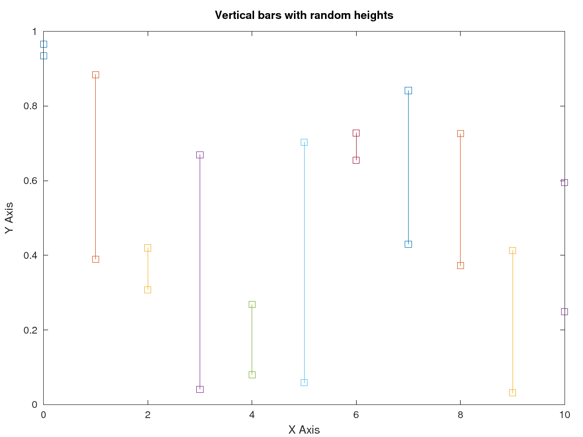
1. Vertical lines with random heights
- x = 0:15;
- plot (repmat (x, 2, 1), rand (2, numel (x)), "-s");
- axis ([0 10 0 1]);
- xlabel("X Axis");
- ylabel("Y Axis")
- title ("Vertical bars with random heights");
- saveas(1, "vertical_bars.png");
Running the code above will result to the figure
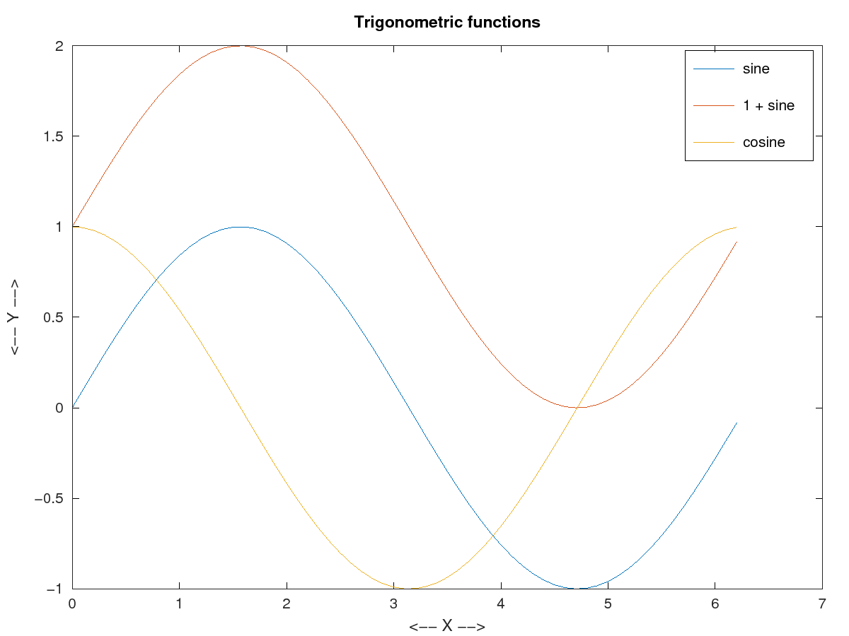
2. Trigonometric functions
- x = 0:0.1:2*pi;
- plot(x, sin(x), "-", x, 1 + sin(x), "--", x, cos(x), ":");
- xlabel("<-- X -->");
- ylabel("<-- Y -->");
- legend("sine", "1 + sine", "cosine");
- title("Trigonometric functions");
- saveas (1, "sine_cosine.png");
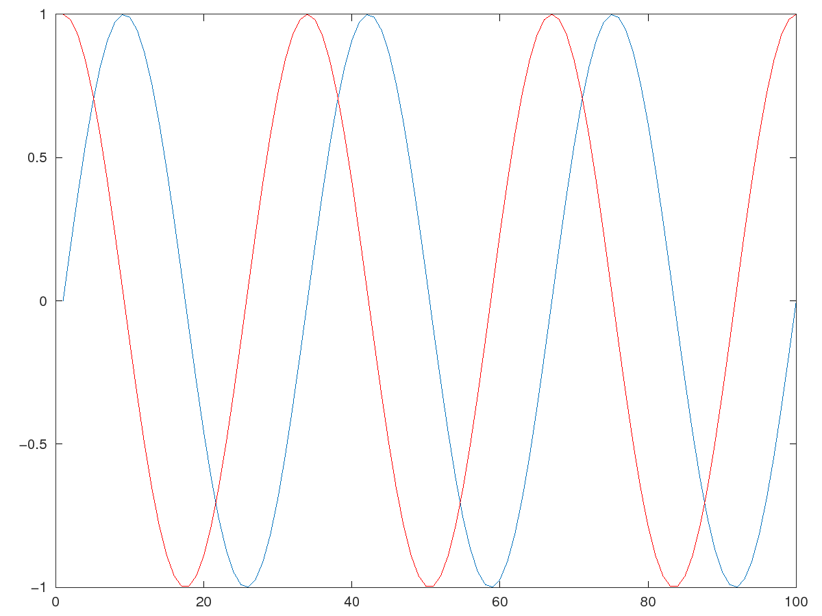
- t = linspace(0,6*pi,100);
- plot(sin(t))
- %grid on
- hold on
- plot(cos(t), 'r')
- saveas (1, "sine_waves.png");
- title("Sine waves")
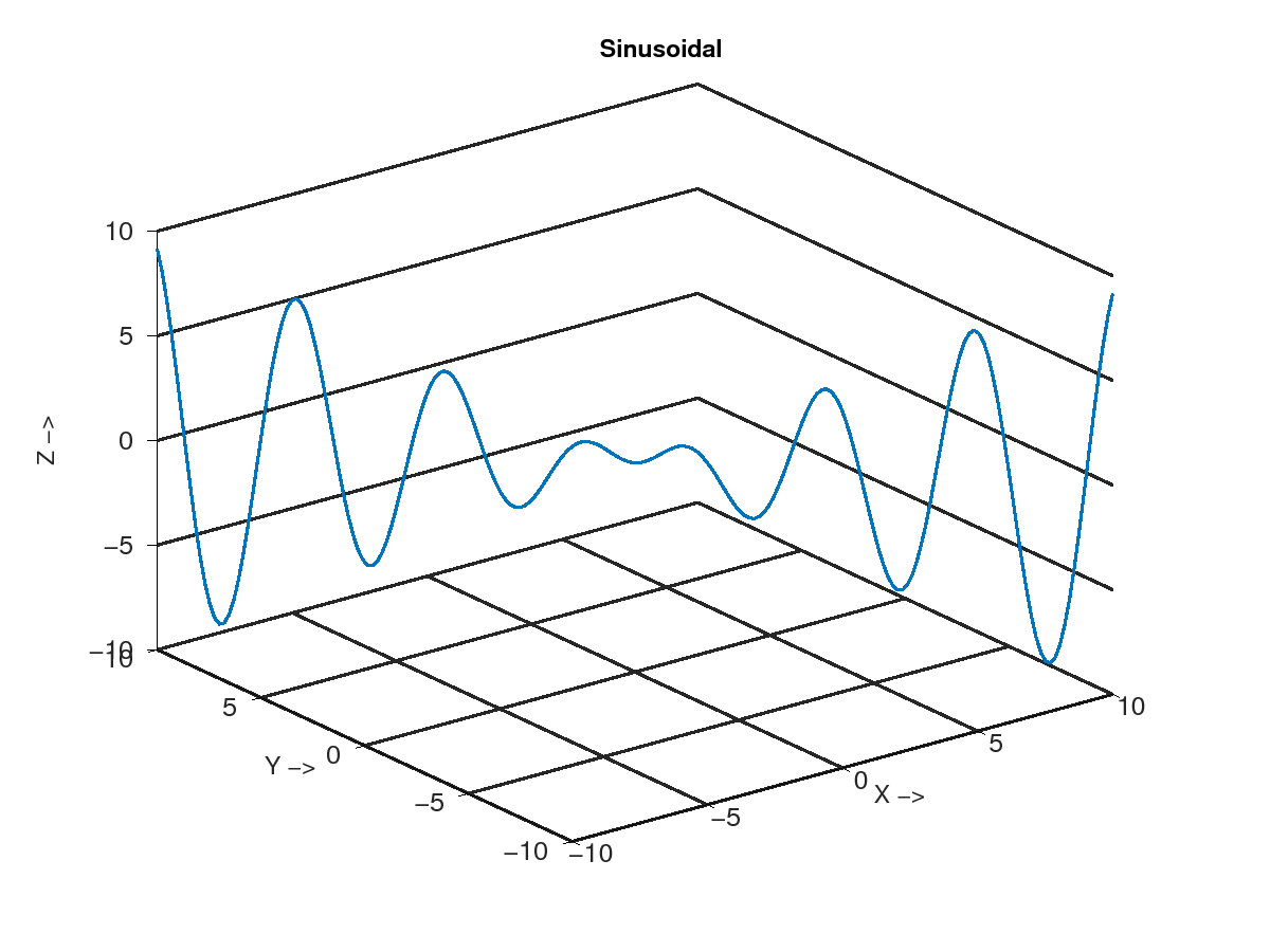
3. Sinusoidal
- x = -10:0.1:10;
- y = 10:-0.1:-10;
- z = x .* sin(x - y);
- plot3(x, y, z, "-", "LineWidth", 4);
- xlabel("X ->");
- ylabel("Y ->");
- zlabel("Z ->");
- title("Sinusoidal");
- set(gca, "linewidth", 4, "fontsize", 12);
- grid("on");
- saveas(1, "Sinusoidal.png")
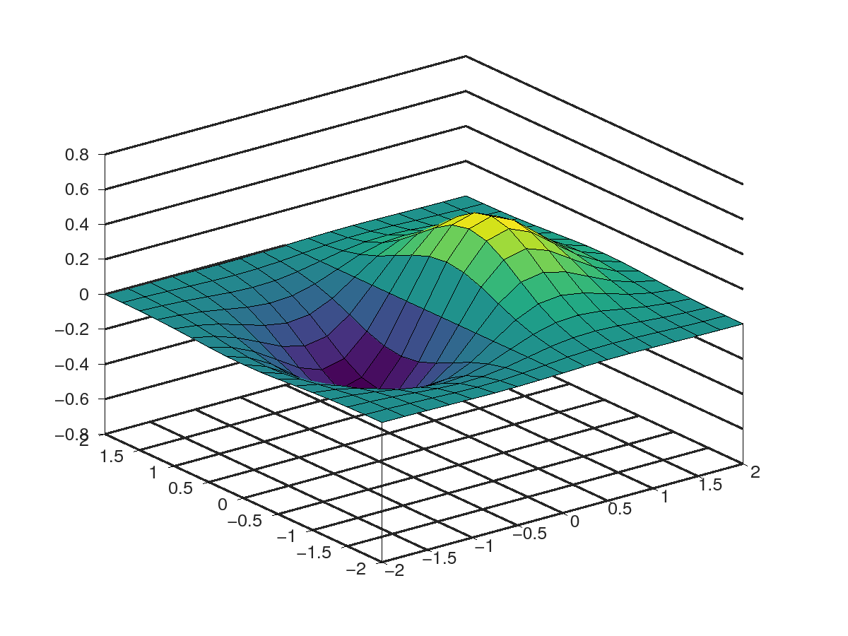
4. Surfaces
- % A 2-D grid with uniformly spaced x-coordinates and y-coordinates in the interval [-2,2]
- x = -2:0.25:2;
- y = x;
- [X,Y] = meshgrid(x);
- F = X.*exp(-X.^2-Y.^2);
- surf(X,Y,F)
- set(gca, "linewidth", 4, "fontsize", 12);
- saveas(1, "surface.png")
- grid on
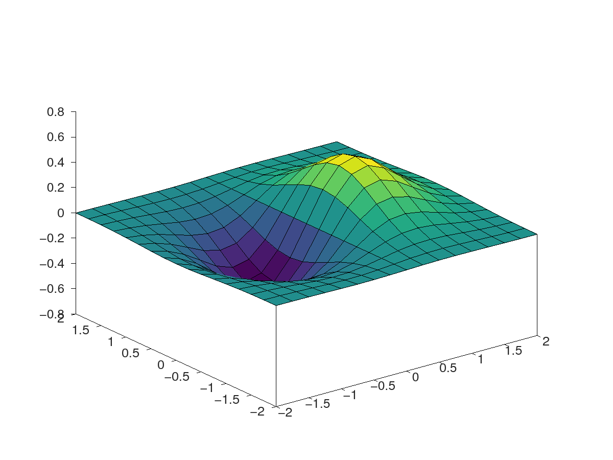
With grids off:
- % Surface - A 2-D grid with uniformly spaced x-coordinates and y-coordinates in the interval [-2,2]
- x = -2:0.25:2;
- y = x;
- [X,Y] = meshgrid(x);
- F = X.*exp(-X.^2-Y.^2);
- surf(X,Y,F)
- set(gca, "linewidth", 4, "fontsize", 12);
- grid("off")
- saveas(1, "no_grid_surface.png")
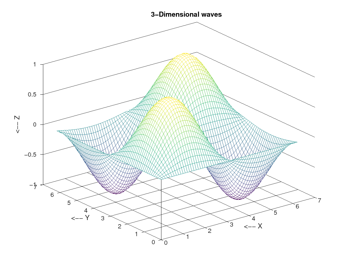
5. 3-Dimensional Graphs
- x = 0:0.1:2*pi;
- y = 0:0.1:2*pi;
- z = sin(x)' * sin(y);
- mesh(x, y, z);
- xlabel("<-- X ");
- ylabel("<-- Y ");
- zlabel("<-- Z");
- title("3-Dimensional waves");
- saveas(1, "3_D_waves.png")
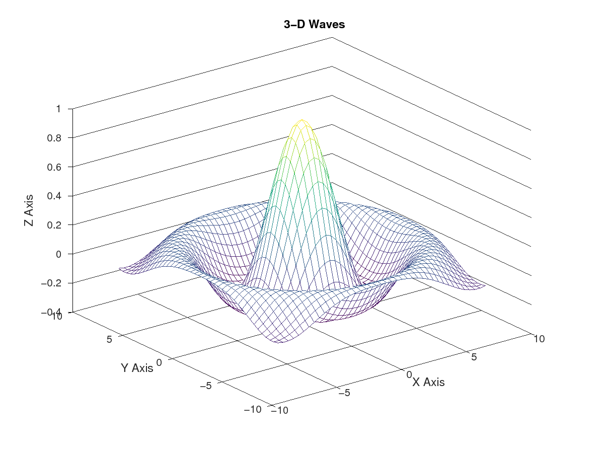
- tx = ty = linspace (-8, 8, 41)';
- [xx, yy] = meshgrid (tx, ty);
- r = sqrt (xx .^ 2 + yy .^ 2) + eps;
- tz = sin (r) ./ r;
- mesh (tx, ty, tz);
- grid on
- xlabel("X Axis")
- ylabel("Y Axis")
- zlabel("Z Axis")
- title("3-D Waves")
- saveas(1, "3_D_waves2.png")
These plots can be greatly enhanced if we use Gnuplot as a plotting engine instead of a default Octave functionality.