The basis of linear regression analysis is to find a straight line (linear equation) that fits or forecasts a set of observations/unobserved values in two dimensions such as all points in a scatter plot which follow or are expected to follow some pattern (usually linear).
Suppose we want to find the relationship between student grades \(y\) and the time \(x\) spent in studying. The linear regression equation of the grade estimates is given by
\begin{equation}
\hat{y} = b_{0} + b_{1}x
\end{equation}
where
- \(\hat{y}\) is the grade estimates,
- \(b_{0}\) is the \(y\) intercept,
- \(b_{1}\) is the gradient/slope of the line. The slope or gradient determines the sensitivity of the dependent variable \(y\) on changes of the values of independent variable \(x\) - how fast/slow the dependent variable varies with an independent variable.
- \(x\) is the student's study time.
\[\begin{array}{|c|c|}
\hline
x&y\\\hline
1&2\\ \hline
2&4\\\hline
3&5\\\hline
4&4\\\hline
5&5\\\hline
\end{array}
\]
We use a simple Python code below to plot the regression line, together with the lines that indicate the means of independent and dependent variables.
- #Import required libraries
- import numpy as np
- import matplotlib.pyplot as plt
- #Create data points
- x = np.array([1,2,3,4,5])
- y = np.array([2,4,5,4,5])
- fig = plt.subplot(111, aspect='auto')
- plt.xlabel("Independent variable x")
- plt.ylabel("Dependent variable y")
- plt.ylim(top=7)
- fig.plot(x, y, 'o', markersize=7, color='black', alpha=1.0, label="Scatter plot")
- plt.axvline(x=np.mean(x), color='red', linestyle='-', alpha=1.0, label="x Mean")
- plt.axhline(y=np.mean(y), color='green', linestyle='-', alpha=1.0, label="y Mean")
- #Fit function
- b1, b0 = np.polyfit(x, y, deg=1)
- f = lambda x: b1*x + b0
- plt.plot(x,f(x), c="purple", linestyle = "-", label="Regression line")
- #Legend, save
- plt.legend(loc=2)
- plt.savefig('regression_line.png', format="png", bbox_inches='tight')
It turns out that the regression line passes through the point where the lines for the means of independent variable \( x \) and dependent variable \(y\) cross, in our case, this point is \((3, 4)\), see the figure below.
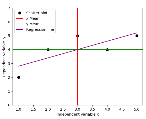
The real world observational data do not always behave linearly. In general, the data will be a series of \(x\) and \(y\) observations (see the table and the figure above), which on average may follow a linear pattern, making it possible to represent them by a linear regression model. However, as we have seen from the figure above, the linear regression line may not always intersect or pass through any of these \((x, y)\) data points, rather, there are going to be errors (that can be measured) due to deviation of data points from the regression line for even the largely unobserved population of values of the independent and dependent variables.
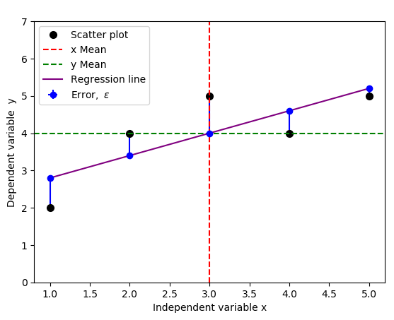
Errors and Error bars
We introduce these errors (or unobserved deviations from the regression line), and denote them as \(\epsilon\), which are distances between the data from the assumed real life (Scatter plot) and the actual linear regression line (purple line). We modify the code above to include and illustrate the errors.
- #Import required libraries
- import numpy as np
- import matplotlib.pyplot as plt
- #Create data points
- x = np.array([1,2,3,4,5])
- y = np.array([2,4,5,4,5])
- fig = plt.subplot(111, aspect='auto')
- plt.title(" ")
- plt.xlabel("Independent variable x")
- plt.ylabel("Dependent variable y")
- plt.ylim(top=7)
- fig.plot(x, y, 'o', markersize=7, color='black', alpha=1.0, label="Scatter plot")
- plt.axvline(x=np.mean(x), color='red', linestyle='--', alpha=1.0, label="x Mean")
- plt.axhline(y=np.mean(y), color='green', linestyle='--', alpha=1.0, label="y Mean")
- #Get intercept and the slope of the fit function
- b1, b0 = np.polyfit(x, y, deg=1)#Fit as first degree polynomial
- f = lambda x: b1*x + b0
- plt.plot(x,f(x), c="purple", linestyle = "-", label="Regression line")
- #Plot half errorbars
- plt.errorbar(x,f(x),xerr=0, yerr=[np.zeros(5), y-f(x)], fmt="o", c="blue", label=r"${\rm Error,} \ \epsilon$")
- plt.legend(loc=2)
- plt.savefig('regression_line_errors.png', format="png", bbox_inches='tight')
The result is the figure below that include the errors, indicated by vertical blue lines:
You could change yerr=[np.zeros(5), y-f(x)] to yerr=[y-f(x), np.zeros(5)] to indicate the opposite errors if needed,
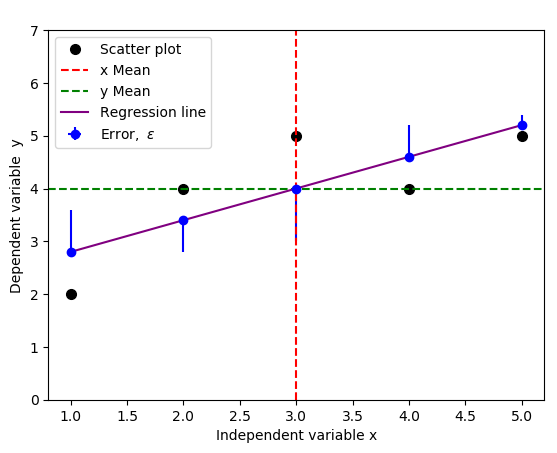
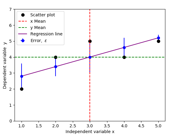
but a standard practice usually includes both negative and positive errors, because we only care about the magnitude of the errors, not direction. You can achieve this by replacing yerr=[np.zeros(5), y-f(x)] with yerr=y-f(x) in the code above:
Depending on your data type and the errors you're interested in, below are few illustrations of typical error bars.
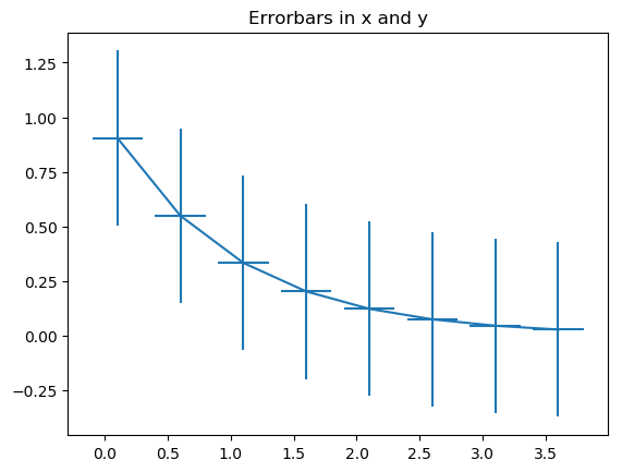
Example 1: error bars in x and y
- import numpy as np
- import matplotlib.pyplot as plt
- #Generate xy data
- x = np.arange(0.1, 4, 0.5)
- y = np.exp(-x)
- #Variable error bar values
- yerr = 0.1 + 0.2*np.sqrt(x)
- xerr = 0.1 + yerr
- #Illustrate basic Matplotlib (can use Pylab) ploting interface
- plt.figure()
- plt.errorbar(x, y, xerr=0.2, yerr=0.4)
- plt.title("Errorbars in x and y")
- plt.savefig('xy_Errobars.png', format="png", bbox_inches='tight')
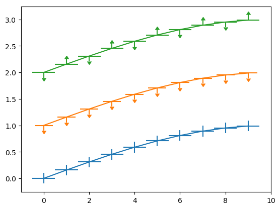
- import numpy as np
- import matplotlib.pyplot as plt
- fig = plt.figure(0)
- x = np.arange(10.0)
- y = np.sin(np.arange(10.0) / 20.0 * np.pi)
- plt.errorbar(x, y,xerr=0.5, yerr=0.1)
- y = np.sin(np.arange(10.0) / 20.0 * np.pi) + 1
- plt.errorbar(x, y,xerr=0.4, yerr=0.1, uplims=True)
- y = np.sin(np.arange(10.0) / 20.0 * np.pi) + 2
- upperlimits = np.array([1, 0] * 5)
- lowerlimits = np.array([0, 1] * 5)
- plt.errorbar(x, y, xerr=0.5, yerr=0.1, uplims=upperlimits, lolims=lowerlimits)
- plt.savefig('Errobars_xy.png', format="png", bbox_inches='tight')
- plt.xlim(-1, 10)
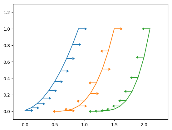
Example 2 : x error bars only
- import numpy as np
- import matplotlib.pyplot as plt
- fig = plt.figure(1)
- x = np.arange(10.0) / 10.0
- y = (x + 0.1)**2
- plt.errorbar(x, y, xerr=0.1, xlolims=True)
- y = (x + 0.1)**3
- plt.errorbar(x + 0.6, y, xerr=0.1, xuplims=upperlimits, xlolims=lowerlimits)
- y = (x + 0.1)**4
- plt.errorbar(x + 1.2, y, xerr=0.1, xuplims=True)
- plt.xlim(-0.2, 2.4)
- plt.ylim(-0.1, 1.3)
- plt.savefig('Errobars_xonly.png', format="png", bbox_inches='tight')
- plt.show()
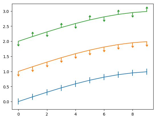
Example 3: y errobars only
- fig = plt.figure(0)
- x = np.arange(10.0)
- y = np.sin(np.arange(10.0) / 20.0 * np.pi)
- plt.errorbar(x, y, yerr=0.1)
- y = np.sin(np.arange(10.0) / 20.0 * np.pi) + 1
- plt.errorbar(x, y, yerr=0.1, uplims=True)
- y = np.sin(np.arange(10.0) / 20.0 * np.pi) + 2
- upperlimits = np.array([1, 0] * 5)
- lowerlimits = np.array([0, 1] * 5)
- plt.errorbar(x, y, yerr=0.1, uplims=upperlimits, lolims=lowerlimits)
- plt.savefig('Errobars_yonly.png', format="png", bbox_inches='tight')
- plt.xlim(-1, 10)
See refs [1], [2].
Thus, a linear regression model must now include this error \(\epsilon\) into it. A simple linear regression model is then given by
\begin{equation}
\hat{y} = b_{0} + b_{1}x + \epsilon.
\end{equation}
This redefined linear regression model can then be used to derive an equation of a line that minimizes these errors. The approach is based on the Least Square Method. The least square method aims to minimize the errors, which are the differences between the actual values (scatter plot points) and estimated values (points along the regression line) and make them small as possible. We show how to use the ordinary least squares (OLS) method below to analytically solve for the slope and intercept estimates and use them to fit a new regression line.
Simple Linear Regression Model - Ordinary Least Squares (OLS): Closed Form Solution
There are inbuilt functions in most of the programming languages such as Python, R, MATLAB and Octave for computing the slope and the \(y\)-intercept estimates from the two-dimensional data points to model a linear regression line. However, we can obtain a closed form solution by defining and minimizing some objective functional. This is done by finding the estimated values \(\hat{b}_{o}\) and \(\hat{b}_{1}\) for the parameters \(b_o\) and \(b_1\) which would provide the best fit for the given two-dimensional dataset. The "best fit" in this case is interpreted as in the least-squares approach - a line that minimizes the sum of squared residuals, \(\hat{\epsilon}_{i}\) (the differences between actual and predicted/estimated values of the dependent variable \(y\)). We can respectively, obtain the \(y\)-intercept and the slope estimates, \(\hat{b}_{o}\) and \(\hat{b}_{1}\) by taking the partial derivative of the objective/cost functional with respect to each term, setting them to zero, and calculate the slope and the \(y\)-intercept, where for the line of a linear regression given by the formula,
\begin{equation}
y_{i} = b_{0} + b_{1}x_{i} + \epsilon_{i},
\end{equation}
we need to find
\begin{align}
\rm{min}_{b_o, b_1} \ F(b_o, b_1)
\end{align}
where
\begin{align}
F(b_o, b_1) & = \sum_{i=1}^{N}(\hat{\epsilon}_{i})^{2}\\
& = \sum_{i=1}^{N}(y_i - b_o - b_{1}x_{i})^{2}.
\end{align}
\(\sum_{i=1}^{N}(\hat{\epsilon}_{i})^{2}\) is called the residual sum of squares (RSS), also known as the sum of squared residuals (SSR) or the sum of squared errors (SSE) of prediction, it explains the deviations of the predicted values from actual empirical values of data. We use this as an optimality criterion for parameter and regression model selection.
We expand the cost functional \(F\) to get quadratic expressions in \(y\)-intercept \(b_o\) and slope \(b_1\),
\begin{align}
F(b_o, b_1) = \sum_{i=1}^{N}(y_{i}^{2} - 2b_oy_i - 2b_1x_iy_i + b_o^{2} + 2b_ob_1x_i + b_1^{2}x_i^{2}),
\end{align}
and then minimize it by taking the partial derivatives of the cost functional \(F\) with respect to \(b_o\) and \(b_1\), setting the results to zero, where finally we have
\begin{align}
F_{b_o} & = \sum_{i=1}^{N}(-2y_i + 2b_o + 2b_1x_i) = 0,\\
& \implies \ \sum_{i=1}^{N}(y_i - b_o - b_1x_i ) = 0.
\end{align}
Therefore,
\begin{align}
\hat{b}_{o} = \bar{y} - \hat{b}_{1}\bar{x} = \dfrac{\sum_{i=1}^{N}y_{i}}{N} - \dfrac{\hat{b}_{1}\sum_{i=1}^{N}x_{i}}{N}.
\end{align}
Similarly,
\begin{align}
F_{b_1} & = \sum_{i=1}^{N}(-2x_iy_i + 2b_ox_i + 2b_1x_i^{2}) = 0,\\
\sum_{i=1}^{N}b_1x_i^{2} & = \sum_{i=1}^{N}(y_ix_i - b_ox_i),\\
b_1\sum_{i=1}^{N}x_i^{2} & = \sum_{i=1}^{N}y_ix_i - \left(\dfrac{\sum_{i=1}^{N}y_i}{N} -b_1\dfrac{\sum_{i=1}^{N}x_i}{N}\right)\sum_{i=1}^{N}x_i,\\
b_1\left(\sum_{i=1}^{N}x_i^{2} - \dfrac{\sum_{i=1}^{N}x_i \sum_{i=1}^{N}x_i}{N} \right) & = \sum_{i=1}^{N}y_ix_i - \sum_{i=1}^{N}y_i\sum_{i=1}^{N}x_i,
\end{align}
which implies
\begin{align}
\hat{b}_{1} & = \dfrac{ \sum_{i=1}^{N}y_{i}x_i - \dfrac{\sum_{i=1}^{N}y_i \sum_{i=1}^{N}x_i}{N}}{\sum_{i=1}^{N}x_i^{2} - \dfrac{\sum_{i=1}^{N}x_i \sum_{i=1}^{N} x_i}{N}}\\[0.3cm]
& = \dfrac{\sum_{i=1}^{N}y_{i}x_i - \bar{y}N\bar{x} - \bar{x}N\bar{y} + N\bar{x}\bar{y}}{\sum_{i=1}^{N}x_{i}^{2} - 2\dfrac{\sum_{i=1}^{N}x_i \sum_{i=1}^{N}x_i}{N } + \dfrac{\sum_{i=1}^{N}x_i \sum_{i=1}^{N}x_i}{N}} \\ \nonumber \\
& = \dfrac{\sum_{i=1}^{N}y_ix_i - \bar{y}\sum_{i=1}^{N}x_i - \bar{x}\sum_{i=1}^{N}y_i + N\bar{x}\bar{y}}{\sum_{i=1}^{N}x_i^{2} -2 \dfrac{\sum_{i=1}^{N}x_i \sum_{i=1}^{N}x_i}{N} + \dfrac{N\bar{x}\sum_{i=1}^{N}x_i}{N}}\\ \nonumber
\\
& = \dfrac{\sum_{i=1}^{N}y_ix_i - \bar{y}\sum_{i=1}^{N}x_i - \bar{x}\sum_{i=1}^{N}y_i + \sum_{i}^{N}\bar{x}\bar{y}}{\sum_{i=1}^{N}x_i^{2} -2 \dfrac{\sum_{i=1}^{N}x_i \sum_{i=1}^{N}x_i}{N} + N\bar{x}^{2}}\\ \nonumber
\\
& = \dfrac{\sum_{i=1}^{N}(x_i-\bar{x})(y_i-\bar{y})}{\sum_{i=1}^{N}x_i^{2} - 2\bar{x}\sum_{i=1}^{N}x_i +\sum_{i=1}^{N}\bar{x}^{2}}\\ \nonumber
\\
& = \dfrac{\sum_{i=1}^{N}(x_i-\bar{x})(y_i-\bar{y})}{\sum_{i=1}^{N}(x_i-\bar{x})^{2}}
\end{align}
Now, we have the \(y\)-intercept estimate,
\begin{align}
\hat{b}_{o} = \bar{y} - \hat{b}_{1}\bar{x} = \dfrac{\sum_{i=1}^{N}y_{i}}{N} - \dfrac{\hat{b}_{1}\sum_{i=1}^{N}x_{i}}{N}
\end{align}
and the gradient estimate,
\begin{align}
\hat{b}_{1} = \dfrac{\sum_{i=1}^{N}(x_i-\bar{x})(y_i-\bar{y})}{\sum_{i=1}^{N}(x_i-\bar{x})^{2}}.
\end{align}
Here,
- \(x_i\) and \(y_i\) are each measurements of two separate attributes of the same observation,
- \(\bar{x}\) and \(\bar{y}\) are respectively, the averages of \(x_i\) and \(y_i\).
\((x-\bar{x})(y-\bar{y})\) is intuitively a vector cross product, and the role of \((x_i-\bar{x})\) and \((y_i-\bar{y})\) is to center values of \(x\) and \(y\) at their means (averages). The multiplication and summation,
\begin{align}
\sum_{i=1}^{N}(x_i-\bar{x})(y_i-\bar{y})
\end{align}
is the dot product of the two vectors \((x-\bar{x})\) and \((y-\bar{y})\) that tells how parallel the two vectors are to each other. More precisely, the dot product of vectors \(x\) and \(y\) can be interpreted geometrically as the length of the projection of \(x\) onto the unit vector \(y\) when the two vectors are placed in such a way their tails coincide (see here).
Now, we're about to introduce the notion of covariance. We can view covariance as the average of the products of the mean deviations \((x_i-\bar{x})\) and \((y_i-\bar{y})\), i.e.,
\begin{align}
\dfrac{1}{N-1}\sum_{i=1}^{N}(x_i -\bar{x})(y_i - \bar{y}).
\end{align}
Covariance of two variables, \(x\) and \(y\) can however be defined by using the notion of expectations (weighted averages of values of \(x\) and \(y\),)
\begin{align}
Cov(x,y) = E[(x-E(x))(y-E(y))],
\end{align}
where \(E\) is the expected value operator.
In general, covariance centers the data to the mean, and the division by \(N-1\) or taking the expected values, is the process of scaling the data by the number of observations. We will see in the subsequent sections how covariance is related to correlation, which is simply a normalized version of covariance.
We can then use the Python code below to calculate the \(y\)-intercept estimate \(\hat{b}_{o}\) and the gradient estimate \(\hat{b}_{1}\).
- def simple_linear_regression(x, y):
- """Returns y-intercept and gradient of a simple linear regression line"""
- #Initial sums
- n = float(len(x)) #We can use x.sum()
- sum_x = np.sum(x)
- sum_y = np.sum(y)
- sum_xy = np.sum(x*y)
- sum_xx = np.sum(x**2)
- #Formula for gradient/slope, b1
- gradient = (sum_xy - (sum_x*sum_y)/n)/(sum_xx - (sum_x*sum_x)/n)
- #Formula for y-intercept, b0
- intercept = sum_y/n - gradient*(sum_x/n)
- return (intercept, gradient)
- x = np.array([1,2,3,4,5])
- y = np.array([2,4,5,4,5])
- print("The y-intercept and gradient are:", simple_linear_regression(x, y))
- The y-intercept and gradient are: (2.2, 0.6)
- #Import required libraries
- import numpy as np
- import matplotlib.pyplot as plt
- #Create data points
- x = np.array([1,2,3,4,5])
- y = np.array([2,4,5,4,5])
- fig = plt.subplot(111, aspect='auto')
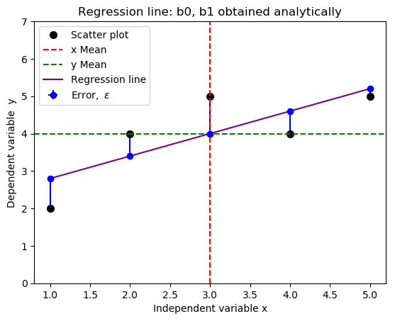
- plt.title("Regression line: b0 and b1 obtained analytically")
- plt.xlabel("Independent variable x")
- plt.ylabel("Dependent variable y")
- plt.ylim(top=7)
- fig.plot(x, y, 'o', markersize=7, color='black', alpha=1.0, label="Scatter plot")
- plt.axvline(x=np.mean(x), color='red', linestyle='--', alpha=1.0, label="x Mean")
- plt.axhline(y=np.mean(y), color='green', linestyle='--', alpha=1.0, label="y Mean")
- #Define the slope and intercept of the fit function
- b1, b0 = 0.6, 2.2
- f = lambda x: b1*x + b0
- plt.plot(x,f(x), c="purple", linestyle = "-", label="Regression line")
- #Plot half errorbars
- plt.errorbar(x,f(x),xerr=0, yerr=[np.zeros(5), y-f(x)], fmt="o", c="blue", label=r"${\rm Error,} \ \epsilon$")
- plt.legend(loc=2)
- plt.savefig('new_fit_regression_line.png', format="png", bbox_inches='tight')
Relationship Between Covariance and Correlation
From the gradient estimate we obtained above,
\begin{align}
\hat{b}_{1} & = \dfrac{\sum_{i=1}^{N}(x_i-\bar{x})(y_i-\bar{y})}{\sum_{i=1}^{N}(x_i-\bar{x})^{2}}\\[0.2cm]
& = \dfrac{\frac{1}{N-1} \sum_{i=1}^{N}(x_i-\bar{x})(y_i-\bar{y})}{\frac{1}{N-1}\sum_{i=1}^{N}(x_i-\bar{x})^{2}}\\[0.2cm]
& = \dfrac{Cov(x,y)}{\sigma^{2}(x)}\\[0.2cm]
& = \dfrac{Cov(x,y)}{Var(x)}\\[0.2cm]
& = \frac{{\rm Sample \ covariance \ of} \ x \ {\text{and}} \ y }{{\rm Sample \ variance \ of } \ x}.
\end{align}
We know that
\begin{align}
{\rm correlation,} \ \ r_{xy} & = \dfrac{Cov(x,y)}{\sqrt{Var(x)Var(y)}} = \dfrac{Cov(x,y)}{\sqrt{Var(x)}\sqrt{Var(y)}}\\[0.2cm]
& = \sqrt{\dfrac{Var(x)}{Var(y)}}\dfrac{Cov(x,y)}{Var(x)}.
\end{align}
\begin{align} {\rm Therefore,} \ \hat{b}_{1} = \dfrac{Cov(x,y)}{Var(x)} = r_{xy}\sqrt{\dfrac{Var(y)}{Var(x)}},\\[0.2cm]
{\Huge \hat{b}_1 = r_{xy}\dfrac{s_y}{s_x}}.
\end{align}
We have introduced new parameters as follows:
- \(Cov(x,y)\), sample covariance of \(x\) and \(y\).
- \(Var(x)\) and \(Var(y)\) are sample variances of \(x\) and \(y\). If a set of data points has many values far away from its mean, it will have a high variance and vice versa.
- \(r_{xy}\), the sample correlation coefficient between \(x\) and \(y\).
- \(s_{x}\) and \(s_{y}\), the sample standard deviations of \(x\) and \(y\). The standard deviation is a measure that is used to quantify the amount/degree of variation or dispersion (how spread) of the set of data values. A small standard deviation means that the data points tend to be close to (clustered around) the mean of the set, while a larger standard deviation means the data points are spread far from the mean.
- The variance is a covariance of a variable, say \(x\), with itself, i.e. \(Cov(x,x) = Var(x)\).
- The square root of variance is called standard deviation.
The solution to these challenges is to normalize the covariance, that's dividing the covariance, \(Cov(x,y)\) by the square root of the product of the variances (standard deviations) of the variables/vectors \(x\) and \(y\). This adjustment represents the diversity and scale in both the covariates, resulting in a value that is certainly between -1 and 1, namely; the correlation coefficient, \(r_{xy}\). Whatever unit the original variables were in, we are assured to always get the same result, and this will also ensure that we can, to a certain extent, compare whether two variables correlate more than two others, simply by comparing their correlation. Very often, correlation, obtained by normalizing (adjusting or standardizing) covariance, is used to compare datasets more easily.
We have seen that covariance simply centers the data. Correlation (dimensionless), however, not only centers the data but also normalizes the data using the standard deviations of the respective variables. Here are few remarks we can make in regard to correlation:
- Positive correlation/relationship means the value of dependent variable increases/decreases as the value of independent variable increases/decreases (\(+1\) means perfectly positively correlated).
- Negative correlation/relationship means the value of dependent variable decreases/increases as the value of independent variable increases/decreases (\(-1\) means perfectly inversely correlated).
- If we get the value of correlation close to zero, it means that the two variables are uncorrelated (zero means perfectly uncorrelated).
The relationship between the Correlation Coefficient, \(r_{xy}\) and the Coefficient of Determination, \(R^{2}\)
From
\begin{align} \hat{y} = \hat{b}_o + \hat{b}_1x\end{align},
Let's substitute the expressions we obtained for the estimates of \(b_o\) and \(b_1\) into the above equation to have,
\begin{align}
\hat{y} & = \bar{y} - \hat{b}_1\bar{x} + r_{xy}\dfrac{s_y}{s_x}x = \bar{y} - r_{xy}\dfrac{s_y}{s_x}\bar{x} + r_{xy}\dfrac{s_y}{s_x}x,\\[0.2cm]
\hat{y} - \bar{y} & = r_{xy}s_{y}\dfrac{x - \bar{x}}{s_x},\\[0.2cm]
\implies \dfrac{\hat{y} - \bar{y}}{s_y} & = r_{xy}\dfrac{x - \bar{x}}{s_x}.
\end{align}
This last equation is in the form \(y = b_o + b_1x\) (linear equation), where \(r_{xy}\) is the slope of the regression line of the standardized data points. Here, the \(y\)-intercept is zero, and hence this regression line passes through the origin.
We can now generalize the notion, \(\bar{x}\), to indicate the average value over the set of random samples, \(x\) and \(y\) as
\begin{align} \overline{xy} = \dfrac{1}{N}\sum_{i=1}^{N}x_iy_i.\end{align}
This notion allows us to construct a formula for \(r_{xy}\), that's
\begin{align} {\Huge r_{xy} = \dfrac{\overline{xy} - \bar{x}\bar{y}}{\sqrt{(\bar{x^{2}} - \bar{x}^{2})(\bar{y^{2}}-\bar{y}^2)}} }\end{align}.
Therefore, we can deduce that, the coefficient of determination, \(R^{2}\) is equal to the correlation coefficient squared, \(r_{xy}^{2}\) for the simple linear regression model with a single independent variable. How? Let's verify this claim mathematically.
From
\begin{align}
\dfrac{\hat{y} - \bar{y}}{s_y} & = r_{xy}\dfrac{x - \bar{x}}{s_x},\\[0.2cm]
r_{xy} & = \dfrac{s_x}{s_y} \times \dfrac{\hat{y}-\bar{y}}{x-\bar{x}},\\[0.2cm]
r_{xy}^{2} & = \dfrac{s_x^{2}}{s_y^{2}}\dfrac{(\hat{y}-\bar{y})^{2}}{(x-\bar{x})^{2}},\\[0.2cm]
r_{xy}^{2} & = \dfrac{\dfrac{\sum_{i=1}^{N}(x_i - \bar{x})^{2}}{N-1}}{\dfrac{\sum_{i=1}^{N}(y_i - \bar{y})^{2}}{N-1}} \times \dfrac{(\hat{y} -\bar{y})^{2}}{(x - \bar{x})^{2}}.
\end{align}
Introducing indices and summation for \((\hat{y} -\bar{y})^{2}\) and \((x -\bar{x})^{2}\), we have
\begin{align}
\implies r_{xy}^{2} & = \dfrac{\dfrac{\sum_{i=1}^{N}(x_i - \bar{x})^{2}}{N-1}}{\dfrac{\sum_{i=1}^{N}(y_i - \bar{y})^{2}}{N-1}} \times \dfrac{\sum_{i=1}^{N}(\hat{y}_i -\bar{y})^{2}}{\sum_{i=1}^{N}(x_i - \bar{x})^{2}},\\[0.2cm]
{\Huge r_{xy}^{2}} & {\Huge = \dfrac{\sum_{i=1}^{N}(\hat{y}_i - \bar{\hat{y}})^{2}}{\sum_{i=1}^{N}(y_i - \bar{y})^{2}} = r_{y\hat{y}}^{2} = R^{2}}.
\end{align}
This analysis can be extended to higher dimensions than 2.
Computing \(R^{2}\)
In regression analysis, \(R^{2}\) tells us how well a regression line predicts the estimates of the actual values. It compares two distances: the distances of actual values from the mean to the distances of estimated values from the mean of the dependent variable \(y\). To calculate \(R^{2}\) from the given dataset, we need to determine:
- the mean of actual values of the dependent variable; in this case, we will use values for the variable \(y\) from the table above with the means, \(\bar{y}\) of \(4\);
- distances of actual values for the depependent variable, \(y\) to the mean, \(y - \bar{y}\);
- distances of estimated values (regression line) to the mean, \(\hat{y} - \bar{\hat{y}}\).
\begin{align} R^{2} = \dfrac{(\hat{y}-\bar{\hat{y}})^{2}}{(y-\bar{y})^{2}}.\end{align}
We summarize this process using the table below.
\[
\begin{array}{|c|c|c|c|c|c|c|}
\hline
x_i& y_i & y_i - \bar{y}_i & (y_i -\bar{y}_i)^{2} &\hat{y}_i & \hat{y}_{i} - \bar{\hat{y}}_{i} & ( \hat{y}_{i} - \bar{\hat{y}}_{i} )^{2} \\
\hline
1&2 &-2 &4 & 2.8& -1.2&1.44 \\
\hline
2& 4&0 &0 &3.4 & -0.6&0.36 \\
\hline
3&5 &1 &1 &4.0 & 0.0 & 0.0 \\
\hline
4& 4&0 & 0& 4.6&0.6 & 0.36\\
\hline
5&5 &1 & 1&5.2 &1.2 &1.44 \\
\hline
\end{array}
\]
Note that, the estimated values, \(\hat{y}\), are computed using the equation \(\hat{y} = b_o + b_1x = 2.2 + 0.6x\), where \(b_0 = 2.2\) and \(b_1 = 0.6\) as we have previously seen. \(\hat{y}\), a predicted value of \(y\) for a given value of \(x\), is the line that minimizes the sum of squared errors, \(\epsilon^{2}\).
We can therefore compute R-squared as follows:
\begin{align} R^{2} & = \dfrac{(\hat{y}-\bar{\hat{y}})^{2}}{(y-\bar{y})^{2}} = \dfrac{\sum_{i=1}^{N}(\hat{y}_i - \bar{\hat{y}})^{2}}{\sum_{i=1}^{N}(y_i - \bar{y})^{2}}\\[0.2cm]
& = \dfrac{1.44 + 0 + 0.36 + 1.44}{4 + 0 + 1 + 0 + 1} = \dfrac{3.6}{6} = 0.6.
\end{align}
\(R^{2}\) is the proportion of the variation in \(y\) being explained by the variation in \(x\).
In most cases, the formula for R-squared is commonly acronymised as
\begin{align}
R^{2} & = \dfrac{\rm ESS/SSR}{\rm TSS/SST} \\[0.2cm]
& = \dfrac{\sum_{i=1}^{N} (\hat{y}_i - \bar{\hat{y}})^{2}}{\sum_{i=1}^{N} (y_i - \bar{y})^{2}},
\end{align}
where,
- ESS/SSR means ESS or SSR, similarly, TSS/SST means TSS or SST.
- ESS is the explained sum of squares, also known as the model sum of squares or sum of squares due to regression ("SSR" – not to be confused with the sum of squared residuals (SSR) that we will explain below).
- The residual sum of squares (RSS), \(\sum_{i=1}^{N}(y_i - \hat{y}_i)^{2}\),
also known as the sum of squared residuals (SSR) ( not to be confused with the sum of squares due to regression "SSR" above) or the sum of squared errors of prediction (SSE). This is the sum of the squares of residuals (sum of deviations of predicted values/estimates from actual empirical/observational data). - TSS is the total sum of squares, alternatively known as sum of the squares (SST), defined as the sum, over all observations, of the squared differences of each observation from the overall mean.
- Generally (see here), the total sum of squares (TSS) = explained sum of squares (ESS) + residual sum of squares (RSS).
Most importantly, don't care much about these terms and their abbreviations, focus on mathematics and how we arrived to \(R^{2}\).
Enjoy maths
Welcome for suggestions and improvements: @Simulink @cache @jiwe @FantasmaDiamato @kipanga @RealityKing @Forbidden_Technology


