Projecting Mollview Maps into Different Coordinate Systems

[Eli]

Python Healpy and Matplotlib are useful tools for plotting and visualization of Mollweide projections. We can use these tools to convert between different Mollview maps, such as Galactic, Ecliptic, Equatorial (Celestial) coordinate systems. Such maps can be very useful in geographical studies that assume the celestial bodies. In Python Healpy (or HEALPIX in general), allowed coordinate systems are 'G' (galactic), 'E' (ecliptic) and 'C' (equatorial). Let's learn by few examples.

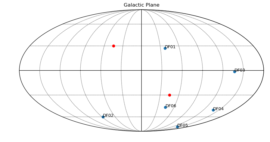
1. Draw a galactic plane and put some labels/objects specified by latitudes and longitudes

Code: [Select all] [Expand/Collapse]

1. import healpy as hp
2. import numpy as np
3. import matplotlib.pyplot as plt #You can import pylab as well
4.  
5. hp.mollview(title="Galactic Plane", norm='hist', xsize=1000)
6. hp.graticule()
7. x = [-37, 88, -137, -139, -136, -44]
8. y = [27, -60, -1.4, -50, -77, -46]
9. lab = ['DF01', 'DF02', 'DF03', 'DF04', 'DF05', 'DF06' ]
10.  
11. hp.projscatter(x, y, lonlat=True, coord="G")
12.  
13. hp.projtext(-37., 27., 'DF01', lonlat=True, coord='G')
14. hp.projtext(88, -60, 'DF02', lonlat=True, coord='G')
15. hp.projtext(-137, -1.4, 'DF03', lonlat=True, coord='G')
16. hp.projtext(-139, -50, 'DF04', lonlat=True, coord='G')
17. hp.projtext(-136, -77, 'DF05', lonlat=True, coord='G')
18. hp.projtext(-44, -46, 'DF06', lonlat=True, coord='G')
19.  
20. equateur_lon = [-45.,45.]
21. equateur_lat = [-30.,30.]
22. hp.projplot(equateur_lon, equateur_lat, 'ro-', lonlat=True, coord='G')
23. plt.savefig("galactic_plane.png", format='png', bbox_inches='tight')

The output should be the galactic plane below



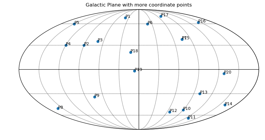
We can plot more or less similar galactic plane as the previous one but with more objects specified on it:

Code: [Select all] [Expand/Collapse]

1. import healpy as hp
2. import numpy as np
3. import matplotlib.pyplot as plt
4.  
5. hp.mollview(title="Galactic Plane with more coordinate points")
6. hp.graticule()
7.  
8. theta =np.array([40.,90.,70.,120.,150.,-20.,-75.,160.,75.,-90.,-127.,-65.,-100.,-160.,-75.,-143.,-72.,13,6.6,-128.])
9. theta = theta.flatten()
10. phi =np.array([70.,30.,35.,30.,60.,60.,38.,-50.,-34.,-52.,-65.,-55.,-30.,-45.,38.,62.,73.,21.,-1.77,-5])
11. phi = phi.flatten()
12. lab = ['P1', 'P2', 'P3', 'P4', 'P5', 'P6','P7', 'P8', 'P9', 'P10', 'P11', 'P12','P13', 'P14', 'P15', 'P16', 'P17', 'P18','P19', 'P20']
13.  
14. hp.projscatter(theta, phi, lonlat=True, coord='G')
15. hp.projtext(40., 70., 'P1', lonlat=True, coord='G')
16. hp.projtext(90., 30., 'P2', lonlat=True, coord='G')
17. hp.projtext(70., 35., 'P3', lonlat=True, coord='G')
18. hp.projtext(120., 30., 'P4', lonlat=True, coord='G')
19. hp.projtext(150., 60., 'P5', lonlat=True, coord='G')
20. hp.projtext(-20., 60., 'P6', lonlat=True, coord='G')
21. hp.projtext(-75., 38., 'P7', lonlat=True, coord='G')
22. hp.projtext(160., -50., 'P8', lonlat=True, coord='G')
23. hp.projtext(75., -34., 'P9', lonlat=True, coord='G')
24. hp.projtext(-90., -52., 'P10', lonlat=True, coord='G')
25. hp.projtext(-127., -65., 'P11', lonlat=True, coord='G')
26. hp.projtext(-65., -55., 'P12', lonlat=True, coord='G')
27. hp.projtext(-100., -30., 'P13', lonlat=True, coord='G')
28. hp.projtext(-160., -45., 'P14', lonlat=True, coord='G')
29. hp.projtext(-75., 38., 'P15', lonlat=True, coord='G')
30. hp.projtext(-143., 62., 'P16', lonlat=True, coord='G')
31. hp.projtext(-72., 73., 'P17', lonlat=True, coord='G')
32. hp.projtext(13., 21., 'P18', lonlat=True, coord='G')
33. hp.projtext(6.6, -1.77, 'P19', lonlat=True, coord='G')
34. hp.projtext(-128., -5, 'P20', lonlat=True, coord='G')
35. plt.savefig("galactic_plane_2.png", format='png', bbox_inches='tight')

And here is the output




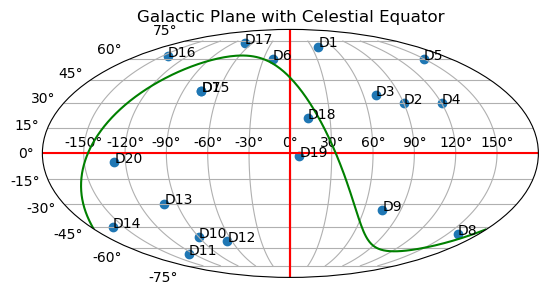
2. You can somehow sophisticate your code and draw a galactic plane, including celestial equator without even using Healpy - only Matplotlib/Pylab

Code: [Select all] [Expand/Collapse]

1. import numpy as np
2. import pylab as plt
3. import math
4.  
5. x =np.array([40.,90.,70.,120.,150.,-20.,-75.,160.,75.,-90.,-127.,-65.,-100.,-160.,-75.,-143.,-72.,13,6.6,-128.])
6. x = x.flatten()
7. y =np.array([70.,30.,35.,30.,60.,60.,38.,-50.,-34.,-52.,-65.,-55.,-30.,-45.,38.,62.,73.,21.,-1.77,-5])
8. y = y.flatten()
9. lab = ['D1', 'D2', 'D3', 'D4', 'D5', 'D6','D7', 'D8', 'D9', 'D10', 'D11', 'D12','D13', 'D14', 'D15', 'D16', 'D17', 'D18','D19', 'D20']
10.  
11. #Plot the celestial equator in galactic coordinates
12. degtorad = math.pi/180.
13. alpha = np.arange(-180,180.,1.)
14. alpha *= degtorad
15. #From Meeus, Astronomical algorithms (with delta = 0)
16. x1 = np.sin(192.25*degtorad - alpha)
17. x2 = np.cos(192.25*degtorad - alpha)*np.sin(27.4*degtorad)
18. yy = np.arctan2(x1, x2)
19. longitude = 303*degtorad - yy
20. x3 = np.cos(27.4*degtorad) * np.cos(192.25*degtorad - alpha)
21. latitude  = np.arcsin(x3)
22.  
23. #We put the angles in the right direction
24. for i in range(0,len(alpha)):
25.     if longitude[i] > 2.*math.pi:
26.         longitude[i] -= 2.*math.pi
27.     longitude[i] -= math.pi
28.     latitude[i] = -latitude[i]
29.  
30. # To avoid a line in the middle of the plot (the curve must not loop)
31. for i in range(0,len(longitude)-1):
32.     if (longitude[i] * longitude[i+1] < 0 and longitude[i] > 170*degtorad and longitude[i+1] < -170.*degtorad):
33.         indice = i
34.         break
35.  
36. #The array is put in increasing longitude
37. longitude2 = np.zeros(len(longitude))
38. latitude2 = np.zeros(len(latitude))
39. longitude2[0:len(longitude)-1-indice] = longitude[indice+1:len(longitude)]
40. longitude2[len(longitude)-indice-1:len(longitude)] = longitude[0:indice+1]
41. latitude2[0:len(longitude)-1-indice] = latitude[indice+1:len(longitude)]
42. latitude2[len(longitude)-indice-1:len(longitude)] = latitude[0:indice+1]
43.  
44. xrad = x * degtorad
45. yrad = y * degtorad
46.  
47. fig2 = plt.figure(2)
48. ax1 = fig2.add_subplot(111, projection="mollweide")
49.  
50. ax1.scatter(xrad,yrad)
51. ax1.plot([-math.pi, math.pi], [0,0],'r-')
52. ax1.plot([0,0],[-math.pi, math.pi], 'r-')
53.  
54. ax1.plot(longitude2,latitude2,'g-')
55. for i in range(0,20):
56.     ax1.text(xrad[i], yrad[i], lab[i])
57. plt.title("Galactic Plane with Celestial Equator")
58. plt.grid(True)
59. plt.savefig("gal_celestial_e.png", format='png', bbox_inches='tight')

The result is



Change -latitude to latitude to have



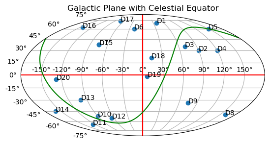
The most important point to note here is, if using Healpy, you can convert between different coordinates by setting the appropriate options: (G[alactic], E[cliptic], C[elestial] or Equatorial=Celestial). Note also, positions are defined by latitudes and longitudes.