KoBo Collect - KoBoToolbox - Google Sheet - TSSFL Stack - Data Analysis

#1

KoBoToolbox is a free and open-source suite of tools for field data collection, very suitable for use in challenging environments. This post intends to teach you how to use KoBoToolbox to collect and submit the data to the KoBo platform using an android device and web-based data collection forms. KoBoToolbox offers two major options for data collection, they are, collecting data using KoBoCollect Android App and data collection using Enketo web forms.

Today we are focusing on Collecting Data with KoBoCollect on Android, and also include all available options for which KoBo forms can be used to collect data, and finally import data from KoBoToolbox into a Google spreadsheet. We further show how to use koboextractor Python module to read data directly from KoBoToolbox and visualize them with various charts.

The procedure to achieve data collection using KoBoCollect Android App goes as follows:

1. Go to KoBoToolbox website and create an account. Confirm/activate the account you created by clicking the link sent to your email. Clicking the link will automatically log you in, otherwise, log in here.

2. After logging in, click the New button on the top left corner to create a new form for your project. You will be presented with four options, choose "Build from scratch". Next, fill in the form details as appropriate.

3. Click the plus (+) sign on the left, write a question, and then click "+ADD QUESTION" on the right to choose a response type from the menu. Let's create a simple form that collects a person's name, age, and height.

4. Select settings to choose whether the question is mandatory or not, or to add skip logic -- that's the condition whether to display the next question or not depending on the previous response. Questions can be grouped and skip logic added to them depending on relevance. You can drag and rearrange questions.

5. Apply validation: a condition for which a certain question/response is valid. Include an error message if the response is not acceptable.

6. Finally, deploy your form. There are multiple options to deploy the KoBo form: we will choose the android application option, and follow these instructions:

Install KoboCollect on your Android device.
Click on three vertical dots (...) to open settings.
Enter the server URL https://kc.kobotoolbox.org and your username and password
Open "Get Blank Form" and select this project.
Open "Enter Data."

Android Application: Configure Kobo Collect, Upload Form, and Collect Data

The whole process is shown pictorially as follows: General Settings -> Server -> Type -> KoBoToolbox, then Get Blank Form, and finally Fill Blank Form:

Other Options to Collect and Submit Data to KoBoToolbox

A. Online-Offline (multiple submission)

This allows online and offline submissions and is the best option for collecting data in the field:

B. Online-Only (multiple submission)

This is the best option when entering many records at once on a computer, e.g. for transcribing paper records.

C. Online-Only (single submission)

This allows a single submission, and can be paired with the "return_url" parameter to redirect the user to a URL of your choice after the form has been submitted

D. Online-Only (once per respondent)

This allows your web form to only be submitted once per user, using basic protection to prevent the same user (on the same browser & device) from submitting more than once

E. Embeddable version

F. View Only

Importing Data From KoBoToolbox Into Google Sheet

We first need to install API Connector: https://gsuite.google.com/marketplace/a ... 5804724197 in order to be able to connect and import data from APIs to Google Sheets. After that, then we can follow these steps:

1. Get your KoBo API key by navigating to https://kf.kobotoolbox.org/token/. This is a string in a double quote that follows after "token":

2. Create your KoBo API request URL, currently the URL is: https://kf.kobotoolbox.org/api/v2/assets.json

3. Pull KoBo API Data Into Google Sheet:

- Open up Google Sheets and click Add-ons > API Connector > Open.
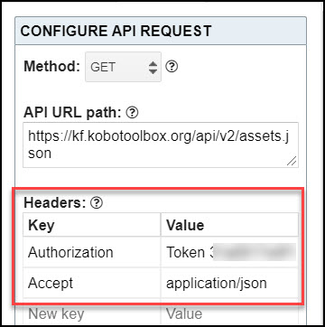
- In the Create screen, enter the API Request URL we just created in 2 above

4. Under Headers, enter two sets of key-value pair like this:

- Authorization: Token Your_API_Token
- Accept: application/json

Only replace YOUR_API_TOKEN with the token you got in 1 above.

5. We don’t need OAuth2 authentication so just leave that set to None. Create a new tab and click ‘Set current’ to use that tab as your data destination.

6. Name your request and click Run. A moment later you’ll see a list of your Kobo assets (forms/projects, questions, blocks, templates, collections) populate your sheet.

We named our request Import From KOBO and this is what we get:

See reference for importing data into Google sheet. See also discussion on KoBo Community.

We can download our data from KoBoToolbox, for example in CSV format, upload it to DropBox, and then retrieve the data for analysis with TSSFL Stack.

#2

See how the deployed forms look like:

#3

We can read KoBo data saved in DropBox as below:

Code: [Select all] [Expand/Collapse]

import urllib.request
import pandas as pd
 
urllib.request.urlretrieve('https://www.dropbox.com/s/ydvnsh33sf9rq5e/KoBo.csv?dl=1', 'KoBo.csv')
 
df = pd.read_csv("KoBo.csv")
#Renaming columns: https://stackoverflow.com/questions/11346283/renaming-column-names-in-pandas
#df2 = df.rename({'What is your name?': 'Name', 'How old are you?': 'Age', 'How tall are you?': 'Height'}, axis=1)  # new method
#df.columns = df.columns.str.replace('What is your name?', 'Name')
print(df)

#4

Let's visualize the Google Sheet data below imported from KoBoToolbox:

Code: [Select all] [Expand/Collapse]

#Plot some graph
#Import required libraries
import gspread
import urllib.request
import numpy as np
import matplotlib.pyplot as plt
import seaborn as sns
import pandas as pd
 
"""
urllib.request.urlretrieve("https://www.dropbox.com/s/mqsyfuetv8potvd/credentials.json?dl=1", "credentials.json")
 
gc = gspread.service_account(filename="credentials.json")
sh = gc.open_by_key("1BC48PKPZW71AC6hOn1SNesvZk1PoBjE4wXwl1YlWFpY") #Open spreadsheet,
#the spreadsheet ID starts with 1019ke.... between "" in the line above
"""
#Alternative
#If your file only has one sheet, replace sheet_url
sheet_url = "https://docs.google.com/spreadsheets/d/1GQk7WzixWPs7iyEwAEm63cMcW6dDX_MzEq0eUKucgEA/edit#gid=0"
url_1 = sheet_url.replace('/edit#gid=', '/export?format=csv&gid=')
 
data = pd.read_csv(url_1)
 
#worksheet = sh.sheet1
 
#Define variables
var1 = "results.Name"
var2 = "results.Age"
var3 = "results.Height"
 
#age = worksheet.col_values(3)[1:]
age = data[var2]
print("Ages:", age)
#height = worksheet.col_values(4)[1:]
height = data[var3]
print("Heights:", height)
 
#Pandas is extremely very useful for Google spreadsheets
#Convert the json to Pandas dataframe
#Get all data records as dictionary
#data = worksheet.get_all_records()
#df = pd.DataFrame.from_dict(data)
 
#Let's get some statistics
#age_arr = np.array(age)
#age_array = age_arr.astype(float)
#h_arr = np.array(height)
#h_array = h_arr.astype(float)
 
print("Average Age:", np.mean(age))
print("Mean Height:", np.mean(height))
print("Minimum and Maximum Age:", np.min(age), np.max(age))
print("Minimum and Maximum Height:", np.min(height), np.max(height))
 
#Let's visualize
#Graph styles and font size
sns.set_style('darkgrid') # darkgrid, white grid, dark, white and ticks
plt.rc('axes', titlesize=18)     # fontsize of the axes title
plt.rc('axes', labelsize=14)    # fontsize of the x and y labels
plt.rc('xtick', labelsize=13)    # fontsize of the tick labels
plt.rc('ytick', labelsize=13)    # fontsize of the tick labels
plt.rc('legend', fontsize=13)    # legend fontsize
plt.rc('font', size=13)          # controls default text sizes
 
#sns list of color plettes
#print(sns.color_palette('deep'), sns.color_palette("pastel"), sns.color_palette("Set2"))
 
#Let's Read Data from Google Sheets into Pandas without the Google Sheets API
#Useful for multiple sheets
sheet_id = "1GQk7WzixWPs7iyEwAEm63cMcW6dDX_MzEq0eUKucgEA"
sheet_name = "Sheet1"
url = f"https://docs.google.com/spreadsheets/d/{sheet_id}/gviz/tq?tqx=out:csv&sheet={sheet_name}"
 
#If your file only has one sheet, replace sheet_url
#sheet_url = “https://docs.google.com/spreadsheets/d/1XqOtPkiE_Q0dfGSoyxrH730RkwrTczcRbDeJJpqRByQ/edit#gid=0"
#url_1 = sheet_url.replace(‘/edit#gid=’, ‘/export?format=csv&gid=’)
 
#Get Pandas dataframe
dataset = pd.read_csv(url)
#print(dataset)
 
#Names = worksheet.col_values(2)[1:]
#Names = data[var1]
#print(Names)
 
df_names = dataset[var1]
df_ages = dataset[var2]
df_heights = dataset[var3]
print(df_names)
 
#Preprocessing
plots = dataset.groupby([var1], as_index=False).mean()
#print(plots)
 
#Bar Plot in MatplotLib with plt.bar()
#Names vs Age
plt.figure(figsize=(10,5), tight_layout=True)
colors = sns.color_palette('pastel')
plt.bar(dataset[var1], dataset[var2], color=colors[:5])
plt.xlabel(var1)
plt.xticks(rotation=90)
plt.ylabel('Age')
plt.title('Barplot')
plt.show()
 
#Name Vs Height
plt.figure()
plt.figure(figsize=(10,5), tight_layout=True)
colors = sns.color_palette('deep')
plt.bar(dataset[var1], dataset[var3], color=colors[:6])
plt.xlabel(var1)
plt.xticks(rotation=90)
plt.ylabel('Height')
plt.title('Barplot')
plt.show()
 
#Bar Plot in Seaborn with sns.barplot()
plt.figure(figsize=(10,5), tight_layout=True)
ax = sns.barplot(x=dataset[var1], y=dataset[var2], palette='pastel', ci=None)
ax.set(title='Barplot with Seaborn', xlabel='Names', ylabel='Age')
plt.xticks(rotation=90)
plt.show()
 
#Barplot grouped data by "n" variables
plt.figure(figsize=(12, 6), tight_layout=True)
ax = sns.barplot(x=dataset[var2], y=dataset[var3], hue=dataset[var1], palette='pastel')
ax.set(title='Age vs Height' ,xlabel='Age', ylabel='Height')
ax.legend(title='Names', title_fontsize='13', loc='upper right')
plt.show()
 
#Histograms with plt.hist() or sns.histplot()
plt.figure(figsize=(10,6), tight_layout=True)
bins = [160, 165, 170, 175, 180, 185, 190, 195, 200]
# matplotlib
plt.hist(dataset[var3], bins=bins, color=sns.color_palette('Set2')[2], linewidth=2)
plt.title('Histogram')
plt.xlabel('Height (cm)')
plt.ylabel('Count')
# seaborn
ax = sns.histplot(data=dataset, x=var3, bins=bins, color=sns.color_palette('Set2')[2], linewidth=2)
ax.set(title='Histogram', xlabel='Height (cm)', ylabel='Count')
plt.show()
 
#Boxplot
plt.figure(figsize=(10,6), tight_layout=True)
ax = sns.boxplot(data=dataset, x=var1, y=var2, palette='Set2', linewidth=2.5)
ax.set(title='Boxplot', xlabel='Names', ylabel='Age (Years)')
plt.xticks(rotation=90)
plt.show()
 
#Scatter plot
plt.figure(figsize=(10,6), tight_layout=True)
ax = sns.scatterplot(data=dataset, x=var2, y=var3,   hue=var1, palette='Set2', s=60)
ax.set(xlabel='Age (Years)', ylabel='Height (cm)')
ax.legend(title='People', title_fontsize = 12)
plt.show()
 
#Something else
pivot = dataset.groupby([var1], as_index=False).mean()
relationship = pivot.loc[:,var2:var3]
print(relationship)
 
#Plot some graph
charts = ["bar", "line", "barh", "hist", "box", "kde", "density", "area"]
for chart_type in charts:
    relationship.plot(kind="%s" % chart_type) #Replace bar with line, barh, hist, box, kde, density, area
    plt.title("%s plot" % chart_type)
    plt.show()
 
#Seaborn
plt.figure()
sns.set_style("darkgrid")
sns.lineplot(data = dataset, x = var2, y = var3)
plt.show()
 
plt.figure()
sns.set_style("whitegrid")
sns.lineplot(data = dataset, x = var2, y = var3)
plt.show()
 
#Hexbin
#Split the plotting window into 20 hexbins
plt.figure()
nbins = 20
plt.title('Hexbin')
plt.hexbin(dataset[var2], dataset[var3], gridsize=nbins, color=colors[:6])
plt.show()
 
#2-D Hist
plt.figure()
plt.title('2-D Histogram')
plt.hist2d(dataset[var2], dataset[var3], bins=nbins, color=colors[:5])
plt.show()
 
#Set variables
x = dataset[var2]
y = dataset[var3]
z = dataset[var1]
 
#Linear Regression
plt.figure()
sns.regplot(x = x, y = y, data=dataset);
plt.show()
 
plt.figure()
sns.jointplot(x=x, y=y, data=dataset, kind="reg");
plt.show()
 
#Set seaborn style
sns.set_style("white")
 
# Basic 2D density plot
plt.figure()
sns.kdeplot(x=x, y=y)
plt.show()
 
# Custom the color, add shade and bandwidth
plt.figure()
sns.kdeplot(x=x, y=y, cmap="Reds", shade=True, bw_adjust=.5)
plt.show()
 
# Add thresh parameter
plt.figure()
sns.kdeplot(x=x, y=y, cmap="Blues", shade=True, thresh=0)
plt.show()
 
#Joint plot
plt.figure()
sns.jointplot(x = x,y = y,data = dataset,kind = 'hex')
plt.show()

#5

Get specific data of the ith asset in your KoBoToolbox account by creating a KoBo API request using a URL of the form https://kf.kobotoolbox.org/api/v2/assets/xxx/data.json where xxx is some string id with the API Connector:

#6

We use koboextract Python module to extract the list of assests and data from KoBotoolbox, and convert kobo data into Pandas DataFrame. We can then process, analyze and visualize the data. This only requires to replace "KoBo_Token" with a valid KoBotoolbox API Key.

Code: [Select all] [Expand/Collapse]

from koboextractor import KoboExtractor #https://pypi.org/project/koboextractor/
kobo = KoboExtractor("KoBo_Token", 'https://kf.kobotoolbox.org/api/v2', debug=True)
 
#Get the unique ID of the ith asset in your KoBoToolbox account:
i = 1
assets = kobo.list_assets()
asset_uid = assets['results'][i]['uid']
 
#Get the list of assets
asset = kobo.get_asset(asset_uid)
#choice_lists = kobo.get_choices(asset)
#questions = kobo.get_questions(asset=asset, unpack_multiples=True)
 
#Download all responses submitted after a certain point in time:
#new_data = kobo.get_data(asset_uid, submitted_after='2020-05-20T17:29:30')
#Get data
new_data = kobo.get_data(asset_uid)
 
#new_data will be an unordered list of form submissions
#We can sort this list by submission time by calling:
 
new_results = kobo.sort_results_by_time(new_data['results'])
#print(new_results)
import pandas as pd
# Create DataFrame
df = pd.DataFrame(new_results)
print("DataFrame:", df.head())
print("KoBo Data Column Names:", df.columns)

#7

The code below does the following: Read data directly from KoBotoolbox, convert the data into pandas dataframe, select a subset of pandas dataframe and upload/paste it into the "imported_from_kobo" sheet of the Kobo_Android_Data Google Spreadsheet below, plot and visualize charts for a select dataset:

Code: [Select all] [Expand/Collapse]

import gspread
import numpy as np
from koboextractor import KoboExtractor #https://pypi.org/project/koboextractor/
kobo = KoboExtractor("KoBo_Token", 'https://kf.kobotoolbox.org/api/v2', debug=True)
 
#Get the unique ID of the ith asset in your KoBoToolbox account:
i = 1
assets = kobo.list_assets()
asset_uid = assets['results'][i]['uid']
 
#Get the list of assets
asset = kobo.get_asset(asset_uid)
#choice_lists = kobo.get_choices(asset)
#questions = kobo.get_questions(asset=asset, unpack_multiples=True)
 
#Download all responses submitted after a certain point in time:
#new_data = kobo.get_data(asset_uid, submitted_after='2020-05-20T17:29:30')
#Get data
new_data = kobo.get_data(asset_uid)
 
#new_data will be an unordered list of form submissions
#We can sort this list by submission time by calling:
 
new_results = kobo.sort_results_by_time(new_data['results'])
#print(new_results)
import pandas as pd
# Create DataFrame
df = pd.DataFrame(new_results)
print("DataFrame:", df.head())
print("KoBo Data Column Names:", df.columns)
 
#Slice a dataframe
dataset = df[["Name", "Age", "Height"]]
#print("df:", df["Age"]=="40")
 
#Convert just columns "Age" and "Height" data types to numerics
df[["Age", "Height"]] = df[["Age", "Height"]].apply(pd.to_numeric)
print("df:", df["Age"]==40)
print("df:", df)
 
#df = df.iloc[:, 2:9]
 
#Select multiple ranges of columns in Pandas DataFrame
df = df.iloc[:, np.r_[2:9, 12:13, 14, 16]]
 
import urllib.request
urllib.request.urlretrieve("https://www.dropbox.com/s/m728v370159b2xm/credentials.json?dl=1", "credentials.json")
 
gc = gspread.service_account(filename="credentials.json")
 
wb = gc.open_by_key("1GQk7WzixWPs7iyEwAEm63cMcW6dDX_MzEq0eUKucgEA")
 
new_sheet = wb.worksheet("imported_from_kobo")
 
new_sheet.update([df.columns.values.tolist()] + df.values.tolist())
 
 
var1 = "Name"
var2 = "Age"
var3 = "Height"
 
#Run code
#Plot some graph
#Import required libraries
import gspread
import urllib.request
import numpy as np
import matplotlib.pyplot as plt
import seaborn as sns
import pandas as pd
 
age = df[var2]
print("Ages:", age)
height = df[var3]
print("Heights:", height)
 
print("Average Age:", np.mean(age))
print("Mean Height:", np.mean(height))
print("Minimum and Maximum Age:", np.min(age), np.max(age))
print("Minimum and Maximum Height:", np.min(height), np.max(height))
 
#Let's visualize
#Graph styles and font size
sns.set_style('darkgrid') # darkgrid, white grid, dark, white and ticks
plt.rc('axes', titlesize=18)     # fontsize of the axes title
plt.rc('axes', labelsize=14)    # fontsize of the x and y labels
plt.rc('xtick', labelsize=13)    # fontsize of the tick labels
plt.rc('ytick', labelsize=13)    # fontsize of the tick labels
plt.rc('legend', fontsize=13)    # legend fontsize
plt.rc('font', size=13)          # controls default text sizes
 
#sns list of color plettes
#print(sns.color_palette('deep'), sns.color_palette("pastel"), sns.color_palette("Set2"))
 
df_names = df[var1]
df_ages = df[var2]
df_heights = df[var3]
print(df_names)
 
#Preprocessing
plots = df.groupby([var1], as_index=False).mean()
#print(plots)
 
#Bar Plot in MatplotLib with plt.bar()
#Names vs Age
plt.figure(figsize=(10,5), tight_layout=True)
colors = sns.color_palette('pastel')
plt.bar(df[var1], df[var2], color=colors[:5])
plt.xlabel(var1)
plt.xticks(rotation=90)
plt.ylabel('Age')
plt.title('Barplot')
plt.show()
 
#Name Vs Height
plt.figure()
plt.figure(figsize=(10,5), tight_layout=True)
colors = sns.color_palette('deep')
plt.bar(df[var1], df[var3], color=colors[:6])
plt.xlabel(var1)
plt.xticks(rotation=90)
plt.ylabel('Height')
plt.title('Barplot')
plt.show()
 
print(df[var1], df[var2])
 
#Bar Plot in Seaborn with sns.barplot()
plt.figure(figsize=(10,5), tight_layout=True)
ax = sns.barplot(x=df[var1].astype("category"), y=df[var2].astype(np.float32), palette='pastel', ci=None)
ax.set(title='Barplot with Seaborn', xlabel='Names', ylabel='Age')
plt.xticks(rotation=90)
plt.show()
 
#Barplot grouped data by "n" variables
plt.figure(figsize=(12, 6), tight_layout=True)
ax = sns.barplot(x=df[var2].astype(np.float32), y=df[var3].astype(np.float32), hue=df[var1].astype("category"), palette='pastel')
ax.set(title='Age vs Height' ,xlabel='Age', ylabel='Height')
ax.legend(title='Names', title_fontsize='13', loc='upper right')
plt.show()
plt.clf()
 
#Histograms with plt.hist() or sns.histplot()
plt.figure(figsize=(10,6), tight_layout=True)
bins = [160, 165, 170, 175, 180, 185, 190, 195, 200]
 
# matplotlib
plt.hist(df[var3], bins=bins, color=sns.color_palette('Set2')[2], linewidth=2)
plt.title('Histogram')
plt.xlabel('Height (cm)')
plt.ylabel('Count')
# seaborn
ax = sns.histplot(data=df, x=var3, bins=bins, color=sns.color_palette('Set2')[2], linewidth=2)
ax.set(title='Histogram', xlabel='Height (cm)', ylabel='Count')
plt.show()
plt.clf()
 
#Boxplot
plt.figure(figsize=(10,6), tight_layout=True)
ax = sns.boxplot(data=df, x=var1, y=var2, palette='Set2', linewidth=2.5)
ax.set(title='Boxplot', xlabel='Names', ylabel='Age (Years)')
plt.xticks(rotation=90)
plt.show()
 
#Scatter plot
plt.figure(figsize=(10,6), tight_layout=True)
ax = sns.scatterplot(data=df, x=var2, y=var3,   hue=var1, palette='Set2', s=60)
ax.set(xlabel='Age (Years)', ylabel='Height (cm)')
ax.legend(title='People', title_fontsize = 12)
plt.show()
 
#Something else
pivot = df.groupby([var1], as_index=False).mean()
relationship = pivot.loc[:,var2:var3]
print(relationship)
 
#Plot some graph
charts = ["bar", "line", "barh", "hist", "box", "kde", "density", "area"]
for chart_type in charts:
    relationship.plot(kind="%s" % chart_type) #Replace bar with line, barh, hist, box, kde, density, area
    plt.title("%s plot" % chart_type)
    plt.show()
 
#Seaborn
plt.figure()
sns.set_style("darkgrid")
sns.lineplot(data = df, x = var2, y = var3)
plt.show()
 
plt.figure()
sns.set_style("whitegrid")
sns.lineplot(data = df, x = var2, y = var3)
plt.show()
 
#Hexbin
#Split the plotting window into 20 hexbins
plt.figure()
nbins = 20
plt.title('Hexbin')
plt.hexbin(df[var2], df[var3], gridsize=nbins, color=colors[:6])
plt.show()
 
#2-D Hist
plt.figure()
plt.title('2-D Histogram')
plt.hist2d(df[var2], df[var3], bins=nbins, color=colors[:5])
plt.show()
 
#Set variables
x = df[var2]
y = df[var3]
z = df[var1]
 
#Linear Regression
plt.figure()
sns.regplot(x = x, y = y, data=df);
plt.show()
 
plt.figure()
sns.jointplot(x=x, y=y, data=df, kind="reg");
plt.show()
 
#Set seaborn style
sns.set_style("white")
 
# Basic 2D density plot
plt.figure()
sns.kdeplot(x=x, y=y)
plt.show()
 
# Custom the color, add shade and bandwidth
plt.figure()
sns.kdeplot(x=x, y=y, cmap="Reds", shade=True, bw_adjust=.5)
plt.show()
 
# Add thresh parameter
plt.figure()
sns.kdeplot(x=x, y=y, cmap="Blues", shade=True, thresh=0)
plt.show()
 
#Joint plot
plt.figure()
sns.jointplot(x = x,y = y,data = df,kind = 'hex')
plt.show()

#8

#9

Mobile data collection using KoBo Collect and KoBoToolbox platform

#10

TSSFL TECHNOLOGY STACK

KoBo Collect - KoBoToolbox - Google Sheet - TSSFL Stack - Data Analysis

Who is online

KoBo Collect - KoBoToolbox - Google Sheet - TSSFL Stack - Data Analysis

Who is online

Login • Register